From Flat Keywords to a Knowledge Graph: Structured Taxonomies for Nature Photography

© 2025 Chris Smith. All rights reserved.

The photo

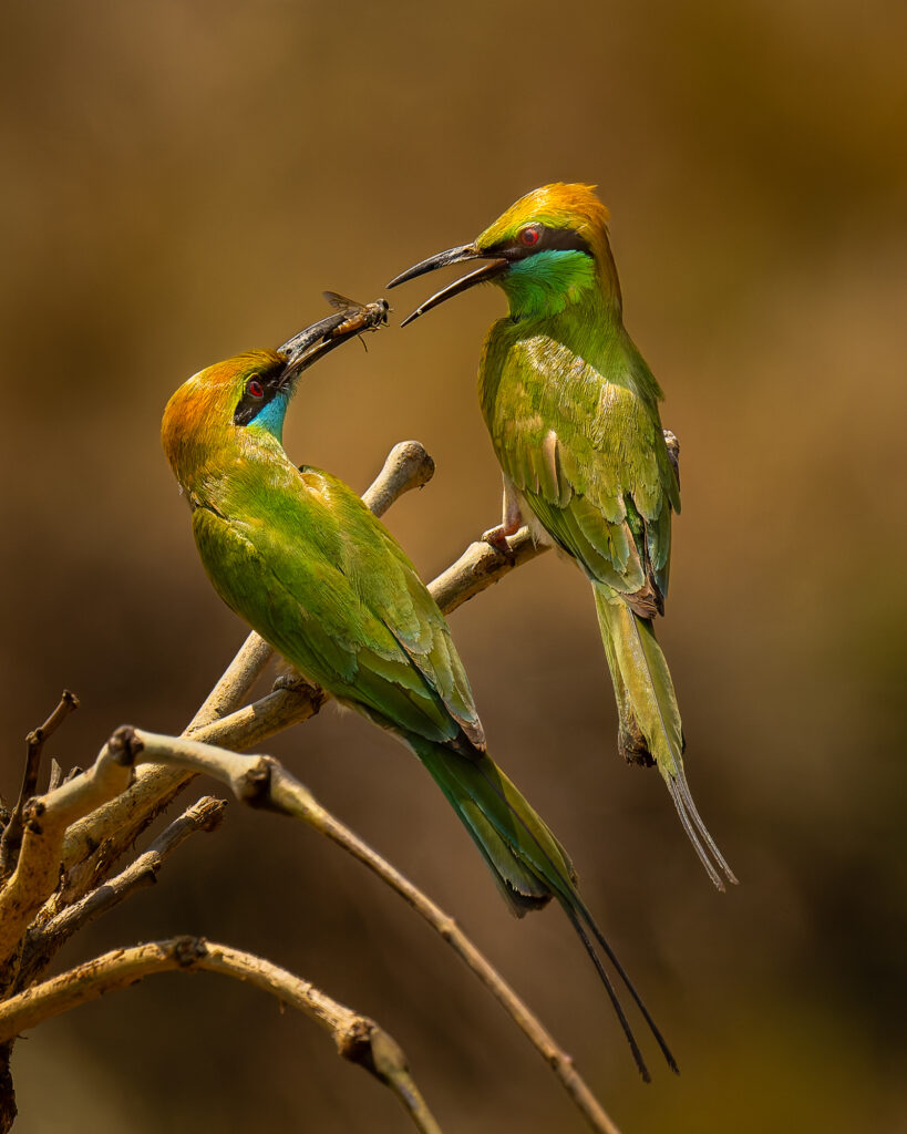
A pair of Asian Green Bee-eaters perched on a bare branch in Kanha National Park, India. One bird is offering an insect to the other — courtship feeding. It’s spring. Kinda harsh, midday light. The GPS coordinates embedded in the image place us in the East Deccan moist deciduous forests ecoregion, in Madhya Pradesh, India.

This photo will gain twelve independent keyword paths by the time it leaves Lightroom. Let’s go through them one group at a time, starting with the taxonomy most folks already understand intuitively.

The idea

Nature photographers are prolific producers of unstructured data. A week in the field yields hundreds or thousands of images, each carrying a handful of camera-generated metadata — shutter speed, aperture, ISO, maybe GPS coordinates if your body supports it. What the camera can’t tell you is that the animal in the frame is a grizzly bear, that you’re standing in the Pacific Temperate Rainforests ecoregion, or that the light right now is technically classified as golden hour. That context lives in your head, and unless you do something deliberate about it, that’s where it stays.

I’ve spent more than two decades working with knowledge graphs and knowledge representation — building systems that make information semantically rich, connected, and discoverable. Many different content and data domains, but none photographic (ask me about Pizza Rat). More than a few years ago, back in the Aperture days, I started applying the same thinking to my nature photography, and it turned out the problem was the same one I’d been solving professionally: valuable information trapped in unstructured form, disconnected from the context that gives it meaning.

These days I shoot wildlife (and occasionally landscape) across the Pacific Northwest, the Rockies, and wherever else I can get to (not as often as I’d like). My keywording system evolved over years. (Probably TMI, but even as a teenager I had a handwritten keyword tagging system – shooting Ektachrome.) Each trip, each new location, each new species added structure, exposed gaps, and sent me looking for better or more authoritative sources – you never want to re-invent an ontology when a de-facto one already exists. Hand-typed place names gave way to geospatial datasets. A partial species taxonomy led to building a full taxonomy – based substantially on data from the Catalogue of Life project. This led to even more data and ontologies that could help me do it right. Eventually I pulled it all together into a cohesive system — a set of independent taxonomies that together describe every photo across its biological, geographic, ecological, temporal, environmental, and cultural dimensions. Each taxonomy is a hierarchy, each hierarchy has a root, and each root maps to a WordPress taxonomy on the portfolio site. When a photo is exported and uploaded, the hierarchical keywords embedded in the image’s metadata are parsed and assigned automatically.

In this post, we trace a single photograph through the entire system to see how structured keywords produce outsized value — and how most of the work is automated.

The problem this solves

More than twenty years of keywording across digital platforms — Aperture, DigiKam, various experiments — had been migrated with varying degrees of success into Lightroom Classic. But, there was a lot of technical debt: place names hand-typed slightly differently across trips, overlapping hierarchies from different eras of thinking about the same problem. None of it was necessarily wrong when it was created — it just reflected a system that had grown organically without a unifying schema.

Travel made it worse – or maybe it was digital (or both). Photographing grizzlies in Alaska one year, British Columbia the next, then Yellowstone in a different season — the geographic and biological scope kept expanding, and the inconsistencies compounded with it. I had an authoritative species taxonomy, but it was unwieldy to apply manually. The place system now needed to work globally and practically it had to be structurally consistent regardless of country or continent. What I had was what you’d call a Folksonomy – what I wanted was a more formal system.

The other piece was having no good way to put the work out there. Social media, in my experience, is a bad form factor for photography — it drives you toward crops, edits, and content choices that serve the platform rather than the subject. The format dictates the presentation, and what works for “the algorithm” isn’t necessarily the image you’d choose as the best representation of what you saw and photographed. Then people would ask “do you have a website where I can see your photos?”, and the answer was no — not for lack of access to platform options, but because I knew what it would take to maintain one properly. The knowledge engineer in me knew that a portfolio site without a coherent metadata system behind it would require constant hand curation to stay current. Every new trip would mean revisiting galleries, re-sorting, re-curating. The site could quickly become stale.

Viewed from the right angle, the keyword mess and the missing website were the same problem: content trapped in a structure that doesn’t match how anyone — photographer or visitor — actually wants to navigate it. Flat keyword lists are one-way doors. They impose a single organizational axis, and finding things any other way means starting from scratch. Faceted navigation solves this problem. You see it every day in e-commerce. It simultaneously allows discovery and provides context for the content you’re viewing. This kind of experience is driven by multiple, related, but non overlapping taxonomies. Each taxonomy describes an independent dimension of a photo — where, what species, what behavior, what light, what ecosystem — and they compose freely. Browse by species this month, reorganize by ecosystem next month, showcase a specific behavior or a specific region, without touching a single photo or re-curating a single gallery.

A system of formal, hierarchical keywords — the same principle behind biological classification — applied systematically to every dimension of a nature photograph. To make that concrete, we’ll follow a single photo through the system and watch the metadata accumulate.

Species: the taxonomy everyone already knows

Most people have at least a passing familiarity with Linnaean classification. Kingdom, phylum, class, order, family, genus, species — it’s the hierarchy behind every field guide (someday we’ll talk taxonomic order, too). It’s also a taxonomy in the formal sense: a structured hierarchy where every entity has a defined position and every position implies a set of parent-child relationships. If you’ve ever thought “that bee-eater is in the kingfisher order,” (because don’t we all?) you’re already thinking in taxonomies.

The species taxonomy in this system is backed by a knowledge graph — a structured model of a domain of knowledge where every entity, relationship, and label is explicitly defined and machine-interpretable. In this case, the domain is the tree of life: every kingdom, phylum, class, order, family, genus, and species, connected by parent-child relationships, with both scientific and common names attached at every level. The knowledge graph is an RDF dataset organized using SKOS (Simple Knowledge Organization System), a W3C standard for representing classification schemes — which means every taxon has a formal scientific name, one or more common names, and a defined position in the hierarchy. It also means that this last sentence is likely only interesting to me, and perhaps two or three other people I know.

The underlying data comes from a comprehensive taxonomy of all life on Earth. Where other, definitive, authoritative sources exist for specific branches, those replace the general-purpose data — the eBird taxonomy from the Cornell Lab of Ornithology provides a widely recognized classification for all birds, for example. The result is complete coverage of the tree of life with specific authoritative sources used where it makes sense.

The workflow in Lightroom: I type a name — common or scientific, full or partial. “Bee-eater,” “Merops orientalis,” or “green bee-eater” all work. (Sometimes the aforementioned field guide is close at hand.) The plugin queries the API, which searches the knowledge graph for exact and fuzzy matches across both scientific and common names. Results are ranked by match quality: exact matches outrank fuzzy ones, and if the query looks like a binomial or trinomial scientific name, species-level matches get priority. This lookup, and applying the keywords to one, or 100, photos, takes only a couple seconds.

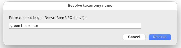
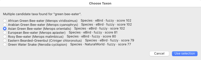
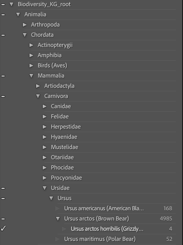
I pick from the ranked candidates, and the API returns the full ancestry — every node from the root through kingdom, class, order, family, and genus, down to the selected taxon. For our bee-eater, that path becomes the first hierarchical keyword on the photo:

Species:              Biodiversity_KG_root | Animalia | Chordata | Birds (Aves)
                        | Coraciiformes | Meropidae (Bee-eaters)
                        | Merops | Merops orientalis (Asian Green Bee-eater)

One taxonomy, one keyword path — and now every photo of an Asian Green Bee-eater is also implicitly tagged as a member of family Meropidae (Bee-eaters), order Coraciiformes, class Aves, and so on up the tree. Browse by family Meropidae on the website and you’ll find green bee-eaters alongside Northern Carmine Bee-eaters, European bee-eaters, and anything else in the family.

The knowledge graph is also a living dataset. A management interface supports adding taxa that don’t exist in the source data, correcting errors, adding common name variants, and creating subspecies under existing species. The grizzly bear subspecies wasn’t in the original data — I added that later (because Ursus arctos horribilis is too fine a subspecies to forgo the latin). The puma (which, incidentally, holds the Guinness World Record for most common names of any mammal) needed several alternative names added before it could be reliably found by some “common” name (I’m looking at you catamount). The knowledge graph grows and improves alongside the catalog.

That’s one keyword path from one taxonomy. I typed a name, selected from ranked candidates (or, if it was definitive, like Grizzly Bear, just a confirmation to use it), and got a full hierarchical classification embedded in the photo. But species identification requires human judgment — you have to know what’s in the frame. What about the dimensions that don’t?

GPS-automatic: the taxonomies that resolve themselves

The bee-eater photo has GPS coordinates embedded in it. From that single data point — a latitude and longitude — the system resolves six more keyword paths without any decision-making required.

The geospatial resolvers work by a common principle: drop a GPS coordinate onto a map of boundaries, and the system tells you what contains that point — which ecoregion, which country, which park, whose traditional lands. The geospatial datasets behind this have been aggregated and curated specifically for nature, wildlife, and conservation photography — global ecoregion boundaries, protected area polygons, administrative divisions, marine water bodies, indigenous territory boundaries. Building and maintaining these datasets is where most of the effort goes. Using them is invisible: the coordinate goes in, the taxonomy paths come out.

Not every camera body has GPS built in, but that doesn’t mean these taxonomies are out of reach. If you record a GPX track on your phone — using Gaia GPS, AllTrails, or any tracking app — the timestamps in the track can be aligned with the photo capture times to retroactively geotag an entire shoot (You can do this with various pieces of software, like exiftool, but I built a plugin for Lightroom that let’s me do it all in one place). The GPS resolvers don’t care how the coordinates got there, only that they’re present.

Here’s what our bee-eater photo gains from its coordinates alone:

Places:               Places_KG_Root | Terrestrial | Asia | Southern Asia
                        | India | Madhya Pradesh | Mandla | Bichhiya

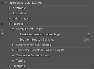
Biogeography:         Ecoregions_2017_KG_Root | Indomalayan
                        | Tropical & Subtropical Moist Broadleaf Forests
                        | East Deccan moist deciduous forests

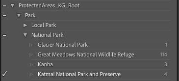
Protected Areas:      ProtectedAreas_KG_Root | Park | National Park | Kanha

Indigenous Lands:     IndigenousLands_KG_Root | Asia | Southern Asia
                        | Gond

Season:               Seasons_KG_Root | Spring

Lighting:             Lighting_KG_Root | Midday

Six keyword paths, six independent taxonomies — all derived from a GPS coordinate and a capture timestamp. Combined with the species lookup, the photo now has seven hierarchical keyword paths. Let’s walk through what each one means.

Places

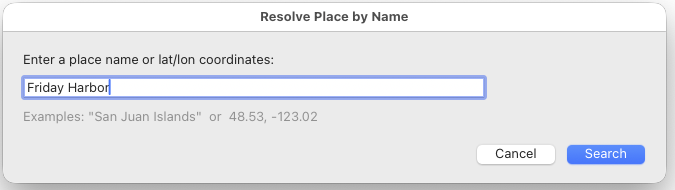
The places taxonomy is the most involved piece of the system because geographic naming is, to put it diplomatically, inconsistent across the world. A single GPS coordinate might fall inside an incorporated city, a county, a state, a country, and a named body of water — and the photographer probably wants all of them represented, in the right hierarchy.

The system handles this by checking multiple spatial datasets in a defined priority order. For terrestrial coordinates, it consults US Census TIGER data (incorporated places and counties), geoBoundaries (a global administrative boundary dataset covering roughly 195 countries), and the UN M49 standard for geopolitical regions and continents. The result is a hierarchical path from continent down to the most specific administrative level available for that location — in practice, this means something like county or municipality in the US, district-level in the UK, commune-level in France, or arrondissement in many countries. The depth varies by country, but the goal is the same: as specific as the data allows.

Coverage is global. Every terrestrial coordinate resolves to at least a continent, country, and first-level administrative unit. Every marine coordinate resolves to at least an ocean (more on that below). Granularity varies: the US has the most detail right now (city and county level from TIGER), while other countries resolve to whatever depth the geoBoundaries data provides. The architecture supports adding more: a new country-specific dataset gets a priority rank, slots into the resolution chain, and the resolver picks the best available source for any given coordinate. The coverage is complete; the granularity is always growing.

For marine coordinates, a separate resolver covers the water. It draws on two sources: OpenStreetMap for named marine features (straits, sounds, bays, fjords, inlets — the kind of detail that matters when you’re photographing from a boat), and the IHO World Seas hierarchy for the larger regional bodies of water. These two datasets have been stitched together into a parent-child hierarchy, so a specific feature like Knight Inlet knows that it sits within a broader sea, which sits within a broader ocean. A photo taken at sea gets both the local detail and the regional context.

My bee-eater photo gets a terrestrial path: Asia > Southern Asia > India > Madhya Pradesh > Mandla > Bichhiya — from continent down to the local administrative level.

Biogeography

The biogeography taxonomy is derived from the WWF Ecoregions 2017 dataset (Olson et al.), a global classification that divides the terrestrial world into 867 named ecoregions, organized by biogeographic realm and biome. The system checks which ecoregion polygon contains the photo’s GPS point.

Ecoregions describe the ecological context that place names can’t. Knowing a photo was taken in Madhya Pradesh tells you the state; knowing it was taken in the East Deccan moist deciduous forests tells you the ecosystem — what kind of forest, what climate regime, what community of species shares that habitat. It’s also the dimension that lets you ask questions across political boundaries: show me everything I’ve shot in tropical moist broadleaf forests, whether that’s central India, Borneo, or the Amazon.

For my Kanha bee-eater photo, the result is the East Deccan moist deciduous forests ecoregion, within the Tropical and Subtropical Moist Broadleaf Forests biome, within the Indomalayan realm. The keyword path captures all three levels.

Most of the time, the GPS point falls cleanly within an ecoregion boundary. Occasionally — for photos taken on a coastline, or on a border between ecoregions — it doesn’t. In these cases, the system finds the nearest ecoregion within a reasonable distance. Beyond that, it returns nothing rather than guessing. Nature photography happens at the edges of things more often than you’d expect (shorelines, treelines, tidal zones), so this fallback matters in practice.

Protected areas — one resolver, four taxonomies

This is where the system does something a bit different. A single resolver queries a combined dataset of the World Database on Protected Areas (WDPA, roughly 300,000 protected areas globally), US National Park Service boundaries, India’s protected areas and tiger corridors, and US Fish and Wildlife Service critical habitat designations. But instead of returning one result, it classifies each matching area into one of four independent taxonomies based on what kind of designation it represents:

• Protected Areas — parks, reserves, refuges, monuments, wilderness areas
• Wildlife Corridors — designated movement and migration corridors
• Landscape Features — formally designated natural features with spatial boundaries
• Conservation Overlays — critical habitat zones, biodiversity hotspots, environmental protection areas

A single GPS coordinate can match areas in more than one of these categories. A point inside Yellowstone National Park falls within a protected area, but it might also fall within designated critical habitat for a specific species (a conservation overlay) and a wildlife corridor. The system checks all four categories in a single pass and returns up to four independent results. Our Kanha photo resolves to a single protected area — the national park itself. Not every photo will trigger all four categories, and most won’t.

Country-specific datasets (US Parks, India’s tiger corridors) take priority over the broader WDPA data for their own geographies. Within a source, the smallest matching area wins — more specific is better. And the proximity threshold is tight (250 meters). Protected area boundaries are often small and precise, and claiming a photo was taken in a national park when it was actually in the adjacent parking lot across the boundary would be a metadata lie.

Indigenous lands

I lived in Australia for a few years, and one of the things that struck me early was how consistently Australians acknowledged the traditional owners of the land. Every public event, every conference, every government website — “We acknowledge the Traditional Custodians of the land…” It was embedded in the culture, a reflexive recognition that the land you’re standing on has a human history that predates your presence by tens of thousands of years. It changed how I thought about place.

A year or two later, working with a photographer and guide in and around First Nations territories in British Columbia — photographing grizzlies in Knight Inlet — that tradition was reinforced.

Nature photography is fundamentally bound to the land — and stewardship of the land and the life it supports has always been central to indigenous peoples. Acknowledging the traditional stewards of the places where we photograph isn’t a detour from the work. It’s part of understanding where you are. So the system does it.

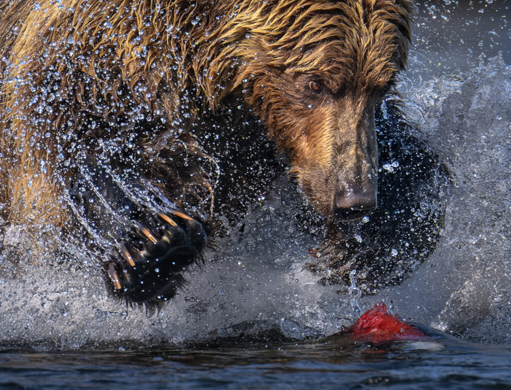
The indigenous lands taxonomy resolves traditional territories from GPS coordinates using the Native Land Digital API, a community-driven dataset that maps indigenous territories, languages, and treaties worldwide. When a photo’s GPS coordinate is sent to the NLD API, it returns the traditional territories that encompass that point. The result is structured into a hierarchy using the same UN M49 regions that the places taxonomy uses for continents and sub-regions — a geopolitically neutral grouping that avoids organizing indigenous territories under colonial state boundaries.

IndigenousLands_KG_Root | Asia | Southern Asia | Gond
IndigenousLands_KG_Root | Americas | Northern America | Yup'ik (Cup'ik)
IndigenousLands_KG_Root | Oceania | Australia and New Zealand | Wurundjeri

The resolver also supports trip-based curation. For locations where the photographer has local knowledge — a guide who named the territory, a land acknowledgment at a lodge, research into the specific peoples of the area — curated territory assignments take priority over the API lookup. The NLD data is a starting point, not the final word. Indigenous territory boundaries are complex, contested, and not always well represented in any single dataset. Where the photographer knows more than the API, the system defers to the photographer.

Our Kanha bee-eater photo resolves to the Gond — one of the largest Adivasi (indigenous) peoples of central India, whose traditional territory spans much of what is now Madhya Pradesh, including the forests that became Kanha National Park.

Season and lighting: the local resolvers

Two of the GPS-automatic taxonomies are computed locally in the Lightroom plugin, with no network call. They need nothing from the API — the GPS coordinates and capture timestamp are sufficient.

Season is the simplest resolver in the system. It uses the photo’s latitude and capture date. Northern Hemisphere, March 20 through June 20 is spring. Southern Hemisphere, the seasons are reversed. The latitude determines which hemisphere’s calendar to use. For a batch of a thousand photos from a week-long trip, all at roughly the same latitude and within the same month, every one of them resolves to the same season in a fraction of a second.

Lighting classifies the ambient light conditions at the moment of capture, computed from the sun’s altitude above (or below) the horizon. Unlike the season resolver, the math is not trivial.

Solar altitude depends on latitude, longitude, date, and time — and crucially, the computation uses the sun’s actual position at those coordinates, not the clock on the wall. This matters more than you might expect. India, for example, uses a single timezone across nearly 30 degrees of longitude — close to two hours of solar time from Gujarat in the west to Arunachal Pradesh in the east. A photo taken at 6:00 AM IST on the western coast and one taken at 6:00 AM IST in the northeast are in very different light. The plugin uses the photo’s GPS coordinates and capture timestamp to compute the sun’s true position using Spencer’s solar declination formula and the equation of time (which corrects for the Earth’s orbital eccentricity and axial tilt). The result is a solar altitude angle in degrees — the actual angle of the sun above or below the horizon at that exact spot, at that exact moment.

That angle maps to a lighting classification:

Condition	Solar Altitude
Night	Below -18°
Astronomical Twilight	-18° to -12°
Nautical Twilight	-12° to -6°
Blue Hour	-6° to -4°
Golden Hour	-4° to 6°
Midday	Above 6°

Golden hour is further split into AM and PM using the solar hour angle — whether the sun is still rising or has started to descend. Every photographer knows the difference between morning and evening golden hour. Now the metadata does too.

So far, our bee-eater has gained seven keyword paths — one from a species search, six from GPS — and I’ve made exactly one decision (selecting the species). Everything else was automatic.

Photographer-applied: the taxonomies that need human eyes

The remaining dimensions require the photographer to make a judgment call. These are things that a GPS coordinate and a species name can’t tell you: what habitat is visible in the frame, what the animal is doing, what kind of photograph the photographer was trying to make.

Seven taxonomies are applied manually in Lightroom, selected from predefined keyword hierarchies that are imported once and then available as click-to-apply keywords. They’re designed to be fast — most photos need a handful of clicks: one for genre, one or two for behavior (if it’s a wildlife shot), one for habitat, and occasionally life stage or sex when they’re identifiable. The keyword hierarchies range from two levels (Sex) to four (Habitat), and the terms are things the photographer already knows from being there.

These aren’t arbitrary categories. Each one is grounded in an established domain.

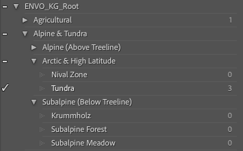
Habitat is based on a simplified version of the Environment Ontology (ENVO), a formal ontology for describing environments. Whether the photo depicts a marine environment, a temperate rainforest, a grassland, or a wetland is something the photographer knows from being there. The GPS coordinate can put you on a coastline, but it can’t tell you whether you’re photographing the tidal zone, the open water, or the cliff above. The hierarchy goes deeper than you might expect — Desert & Arid alone branches into hot desert, high desert, sagebrush steppe, badlands, and lava fields, each a distinct environment that a photographer would recognize on sight.

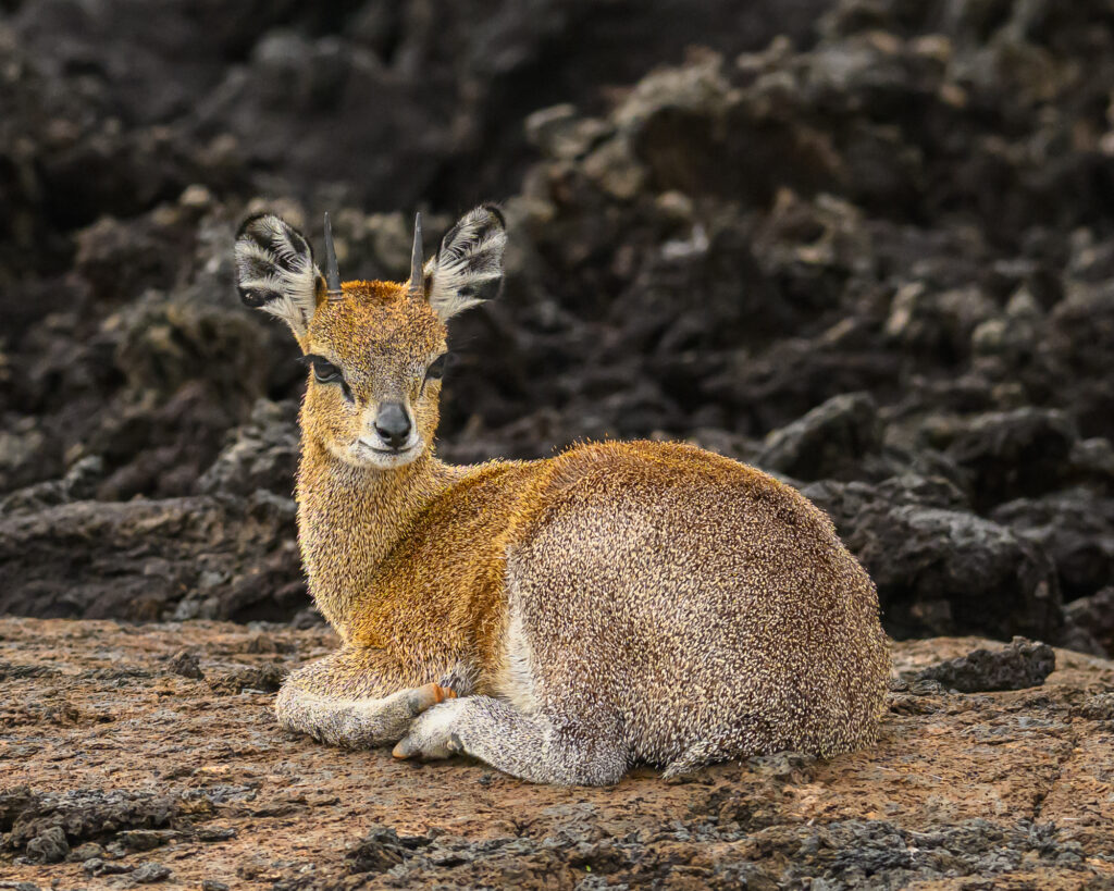
Landscape Features captures the physical geography and notable structures visible in or relevant to the frame. The taxonomy has two branches: Natural — waterfalls, fjords, glaciers, old-growth stands, tide pools, rivers, meadows — and Built — bridges, monuments, lighthouses, places of worship. The type hierarchy provides the classification: a photo tagged under Waterfalls is a waterfall photo regardless of which waterfall. But the taxonomy also accommodates named features — Brooks Falls, the Mara River, Indian Creek — added as children of their type when the specific feature matters. Sometimes the feature is the subject. Sometimes it’s ecological context — the creek beneath a heron rookery, the ridge a hawk migration follows. Either way, it’s the kind of geographic specificity that administrative place names can’t capture. The GPS resolver will tell you the county; it won’t tell you the creek. Not every photo needs a landscape feature — our bee-eater shot doesn’t — so the taxonomy simply isn’t applied.

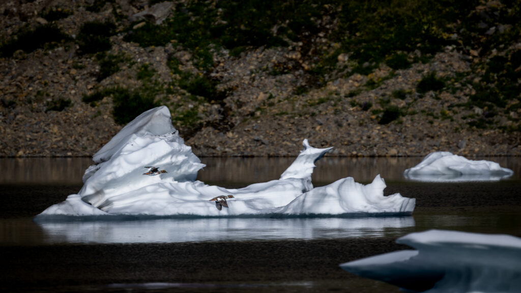
Genre describes the photographer’s intent — what kind of image they were trying to make. The same species in the same location can produce a wildlife portrait, an action shot, or a behavioral study depending on composition and what story the image tells. The genre hierarchy covers wildlife (portraits, birds in flight, action, group), landscape (grand, intimate, seascape, nightscape), macro, astrophotography, underwater, and documentary work. Our bee-eater courtship scene is a wildlife portrait.

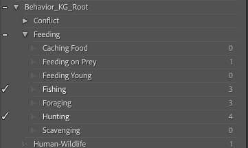
Behavior describes what the animal is doing. Feeding (hunting, fishing, foraging), locomotion (flying, swimming, climbing), social behaviors (courtship, parenting, play), resting, and interactions (conflict, predation, symbiosis). This is the most valuable manual tag for discoverability — people search for “bee-eater courtship” or “eagle hunting,” and the behavior taxonomy makes those searches work at the taxonomy level, not as free-text keyword guesses. Our photo gets Social > Courtship & Display.

Life Stage classifies the animal’s age and maturity: adult (breeding or non-breeding condition), subadult, juvenile (yearling, COY, fledgling, nestling). A grizzly sow with cubs of the year would get both “Adult” and “COY” applied. A bull elk in September velvet gets “Adult > Breeding Condition.” Our bee-eaters are both adults.

Sex — male or female, tagged only when visually determinable and relevant. Antlered elk, maned lions, dimorphic bird plumage. When you can’t tell, you don’t tag it.

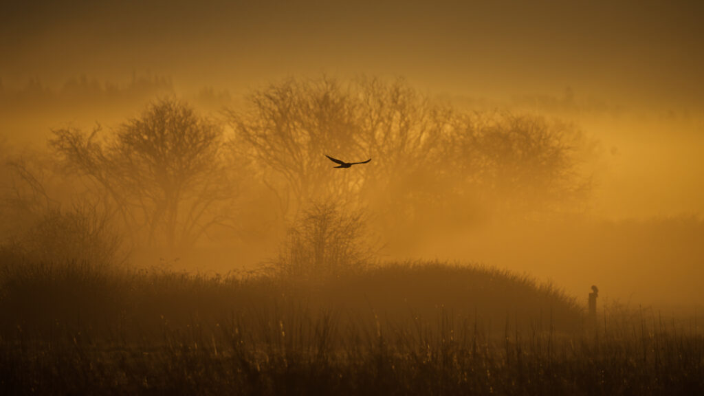
Weather describes weather phenomena when they’re a significant element or subject in the photograph — not the ambient conditions during the shoot, but weather you can see in the frame. Fog rolling through a valley, a cumulonimbus anvil towering over a prairie, lightning, a rainbow after a storm, rime ice on a ridgeline. The hierarchy covers fog, cloud types (from lenticular to mammatus to noctilucent), storms (supercell, tornado), precipitation, and frost formations. Most wildlife photos don’t need a weather tag. When the weather is the story — or half the story — this taxonomy captures it.

Capture Technique — tagged when the photographic method is notable: long exposure, focus stack, panorama, aerial, flash, camera trap. Most photos are straightforward single exposures and don’t need this tag. When the technique contributes meaningfully to the image, the taxonomy lets you record it.

Here’s what I add to our bee-eater with a few seconds of clicking:

Habitat:              ENVO_KG_Root | Forest & Woodland
                        | Climate & Moisture Regime | Tropical Dry Forest
Genre:                Genre_KG_Root | Wildlife | Wildlife Portrait
Behavior:             Behavior_KG_Root | Social | Courtship & Display
Life Stage:           LifeStage_KG_Root | Adult
Sex:                  Sex_KG_Root | Male
                      Sex_KG_Root | Female

All seven manual taxonomies use the same hierarchical keyword structure and travel through the same export pipeline as the automated ones. The only difference is who decides which keywords to apply.

The complete picture

Our bee-eater photo now carries twelve independent keyword paths: one from a species search, six resolved automatically from GPS, and five tagged by the photographer. Not every photo lights up every taxonomy — this image doesn’t have wildlife corridors, conservation overlays, landscape features, weather, or a notable capture technique, because none of those dimensions apply. The system doesn’t force keywords where they don’t belong.

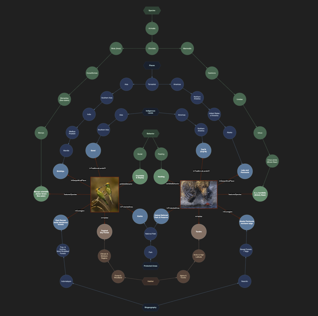
In total, the system uses seventeen independent taxonomies. Nine resolve automatically from GPS coordinates. One comes from a species search. Seven are applied manually in a few clicks. All of them are embedded in the image’s XMP metadata when the photo leaves Lightroom, and all of them are parsed into WordPress taxonomy terms when the photo is uploaded to the site.

Why orthogonal facets matter

Traditional photo tagging tends toward a single hierarchy: Location > Country > State > Park > Species. This looks tidy until you need to ask a question that crosses categories. How many species have I photographed in national parks? Which ecoregions overlap with which protected areas? What’s the most common lighting condition in my coastal photos?

With a single hierarchy, these questions require brittle workarounds or custom queries. With orthogonal facets — independent taxonomies that each describe a different dimension of the photo — they’re straightforward filters. Show me everything in Ursidae (species) AND Pacific Temperate Rainforests (biogeography) AND Autumn (season) AND Feeding (behavior), and you get exactly what you’d expect. No taxonomy needs to know about any other taxonomy. They compose.

This is the same principle behind faceted classification in library science, and behind dimensional modeling in data warehousing. It’s not a new idea. It’s a good one that somehow hasn’t made it into most photographers’ metadata workflows, probably because building the infrastructure to support it is more work than most people want to take on. (I might have underestimated that scope myself, initially.)

From Lightroom to the web

The pipeline that moves these keywords from a photo in Lightroom to a browsable, searchable taxonomy on the website has three stages — and the photographer never leaves Lightroom until the photos are live on the site.

In Lightroom Classic, each taxonomy is represented as a hierarchical keyword tree. The plugin resolves the automated taxonomies — a batch operation that processes an entire shoot’s worth of photos at once — and the photographer applies the manual ones. When the photos are ready, the Lightroom export plugin publishes them directly to WordPress. There’s no separate upload step, no FTP, no media library drag-and-drop. Select photos, hit export, and they go to the site with all their metadata intact.

On the WordPress server, a plugin reads each uploaded image’s embedded metadata — the EXIF and XMP data that Lightroom wrote into the file. It finds the hierarchical keyword paths, identifies each root keyword, maps it to the corresponding WordPress taxonomy, and creates the full parent-child term hierarchy if it doesn’t already exist. The photo is then assigned to the most specific term in each taxonomy. This is invisible to the photographer — the export lands, the taxonomy assignments happen, and the photo is browsable on the site within seconds.

On the website, the taxonomies serve two very different purposes depending on who’s looking.

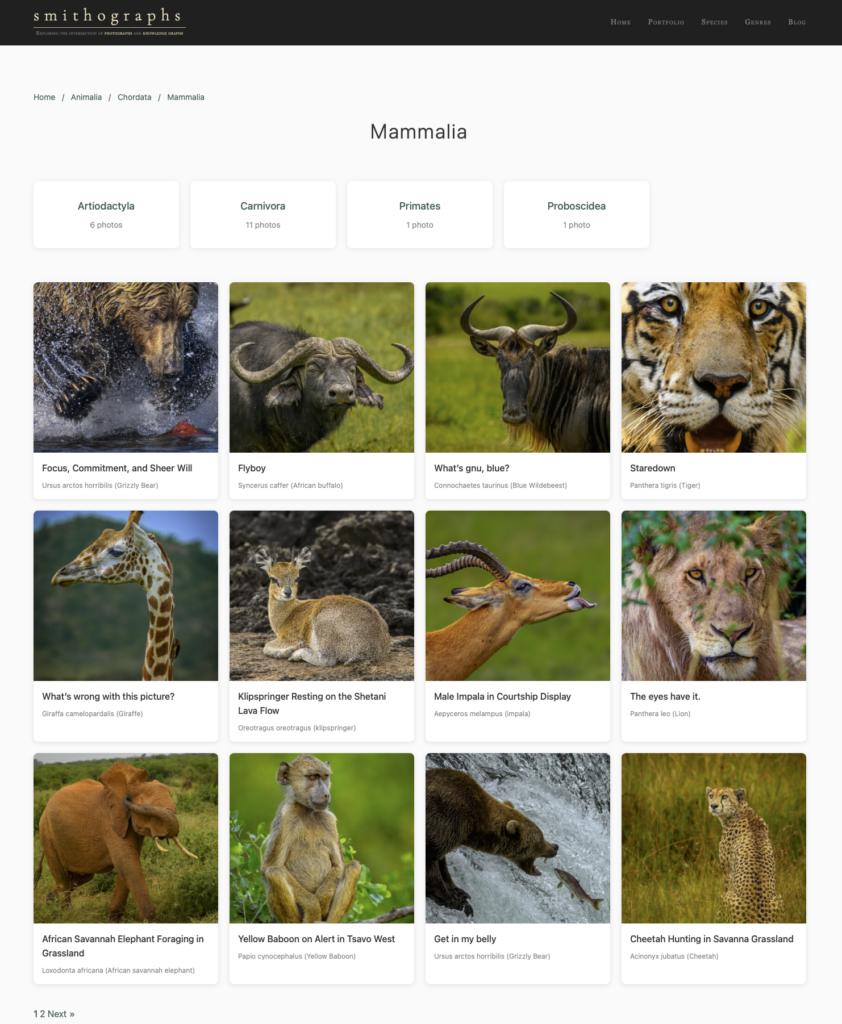
For visitors, the site offers faceted browsing. Each taxonomy has its own archive pages. Visit /species/merops-orientalis/ and you see every Asian Green Bee-eater photo. Visit /biogeography/east-deccan-moist-deciduous-forests/ and you see everything shot in that ecoregion — bee-eaters, tigers, langurs, landscapes. Visit /indigenous-lands/gond/ and you see every photo taken on Gond lands. Breadcrumbs show the hierarchy. Sidebar navigation shows siblings and parents. Visitors can combine facets to narrow their view: bee-eaters in spring, courtship behaviors in national parks, Meropidae across all ecoregions.

For the photographer, the taxonomies are a gallery curation tool. This is where the system changes the workflow most. Traditional portfolio sites require the photographer to manually select and arrange photos into galleries — “Best of India,” “Birds of Kanha,” “Spring Wildlife.” It’s tedious work, it doesn’t scale, and every new photo means revisiting every gallery it might belong in.

With faceted taxonomies, a gallery is a query. “Bee-eaters in Indian national parks” isn’t a hand-curated collection — it’s a facet intersection: Species > Meropidae + Protected Areas > National Park + Places > India. Define the gallery once, and every photo that matches the criteria appears in it automatically. New photos from a future trip show up the moment they’re published. Galleries can be hierarchical — an “India Wildlife” gallery contains “Kanha National Park” as a sub-gallery, which contains “Birds of Kanha” within it. The photographer controls what visitors see, but the taxonomy does the curation.

What this enables

The point of this infrastructure isn’t metadata for metadata’s sake. It’s to make a photo archive that you can ask questions of — and that the web can ask questions of, too.

A visitor can browse by species and discover the ecoregions and protected areas where those species were photographed. They can start from a behavior — courtship — and see which species and locations are represented. They can filter by season and lighting to find golden-hour autumn shots or midday tropical scenes. Each taxonomy is an independent entry point into the collection, and because the taxonomies are hierarchical, browsing at any level works. You can look at all birds, narrow to order Coraciiformes, or go straight to Merops orientalis.

For search engines, the structured taxonomy data generates Schema.org markup on every photo page — explicit, machine-readable statements about what each photograph depicts, where it was taken, and in what ecological context. Most photography portfolios offer a title, a date, and maybe a location tag. A page on this site carries structured data for species, place, ecoregion, protected area, indigenous territory, season, lighting, habitat, behavior, and more. That’s the kind of semantic density that search engines reward with rich results and that AI systems can cite in generated answers.

For AI retrieval — the systems behind ChatGPT, Perplexity, and Google’s AI overviews — structured, authoritative content with specific claims and consistent entity naming is exactly what gets surfaced. A page that says “Merops orientalis courtship feeding photographed in the East Deccan moist deciduous forests ecoregion, Kanha National Park, Madhya Pradesh, during spring” is content that AI models can extract, cite, and link to. It’s specific enough to be useful and structured enough to be machine-readable. Most photography sites offer neither.

The datasets behind the system are global in scope — 867 ecoregions, 300,000+ protected areas, administrative boundaries for 195 countries, marine coverage from the IHO and OpenStreetMap, indigenous territory boundaries from Native Land Digital, and a species knowledge graph covering the tree of life from kingdom to subspecies. The photography catalog grows one trip at a time, but the infrastructure is ready for wherever the next trip goes.

Building a seventeen-taxonomy knowledge graph for a photography portfolio took more effort than any reasonable person would recommend. But the hard part was building it. Using it — type a species name, click resolve, batch-process GPS coordinates, tag a few behaviors and a genre, publish directly from Lightroom — takes less time per photo than most photographers I know spend on basic keywording. The galleries define themselves. The structured data writes itself. The archive gets smarter with every photo added.

For someone who has spent 20+ years making information findable, and who photographs the natural world, it turns out to be worth the trouble.